Excel Text Functions (II) - Extracting text strings using LEFT, RIGHT and MID

LEFT, RIGHT and MID are the three Excel Functions allow users to extract portions of strings from different positions.

(I) LEFT
LEFT returns a specified number of characters, starting from the left most character of the string:

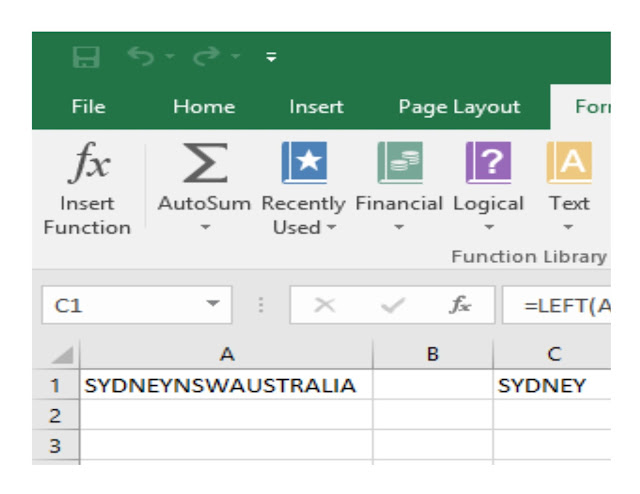
In this example, we are using a sample text string "SYDNEYNSWAUSTRALIA" which is in cell A1.

First of all, we have to go to "Formulas" tab, select "Text" which activates a drop-down list, from which we highlight and select "LEFT".

Once "LEFT" was selected, the "Function Arguments" dialog box will pop up:

User can either enter the text string directly into the "Text" box or clicking the small box at the right which will activate another dialog box as follows:

By clicking cell A1, Excel will put that cell reference into the "Text" box as shown below:

Next, user have to tell Excel how many characters from the left should be extracted, this is done by entering that number of characters into the "Num_chars" box. In our example, we enter 6 which means we will extract 6 characters from the left, following is the result:

(II) RIGHT

RIGHT returns a specified number of characters starting from the rightmost character of the string.

Similar to LEFT, user also access RIGHT by going to "Formulas" tab, select "Text" which activates the drop-down list, from which highlight and select "RIGHT", which will activate the "Function Arguments" dialog box as follows:

We are still using the text string in A1, the number of characters is 9, following is the result:

(III) MID

MID is the function that will return a specified number of characters starting from a specified position.

MID is also located under "Formulas" tab => "Text". From the drop-down list, we highlight and select "MID", which activates the Mid "Function Arguments" box:

We are still using the sample text in cell "A1" as our text string, the "Start_num" is 7, and the "Num_chars" is 3, following is the result:

Excel Text Functions (I) - Concatenating text strings

"CONCAT" (Excel 2016) or "CONCATENATE" (earlier versions) is the Excel function used to join two or more text strings into one.

The basic Syntax of CONCAT:

CONCAT (X1, X2, ...)

The arguments can be text strings or their respective cell references, and users can also add commas, hyphens, spaces, etc., to custom and format the resulting text. Following is an example:

Our arguments include 5 text strings located in cells A1 to A5, in between them we have added three spaces and one comma. The resulting string is as follows (at cell A7):

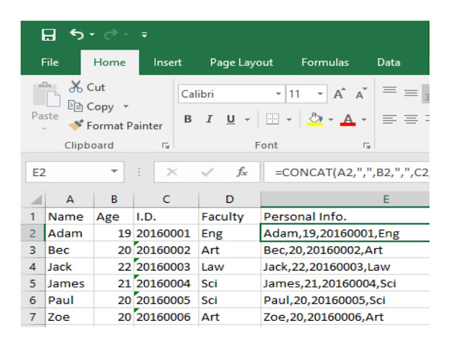
The function can expand to concatenate data in cells of different columns:

By copying formula in E2, we can easily extend the concatenating actions towards other rows:

Pivot Table - Customizing and Formatting

Sum or Count
When creating a pivot table, Excel will automatically sum or count the items. If all the cells in a column contain numeric data, Excel chooses to sum. However, if one cell is either blank or contains text, Excel will choose to count.

To overwrite the default:

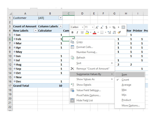
Right click any cell of the column that need to be changed, from the drop-down list, choose "Summarize Values By", from the fly-out menu click "Sum", then the pivot table will sum the items as follows:

Replacing Blanks with Zero
By default, pivot table will leave empty cells blank. To avoid values columns been treated as text just because of one blank cell, we can replace the blank cells with zeros:

Right click any cell of that specific column, choose Pivot Table Options:

A "Pivot Table Options" window will be activated:

In the pop up window, under Layout and Format tab, go to Format, type "0" into the box next to the field "For empty cells show".

Grand Totals
The default in Pivot Table is to show "Grand Total" for both rows and columns:

If user just want Grand Total rows, but not Grand Total columns, that can be done as follows:

Go to Design tab => Select Grand Totals =>Select "On For Rows Only" from the drop-down list

The drop-down list offers 4 choices: users can also choose "On for Columns Only", or on and off for both.


Subtotals
There are times users need to suppress the subtotals. To do so, user can go to Design tab, then

click Subtotals, from the drop-down list, select Do Not Show Subtotals.

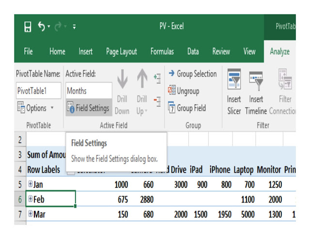
However, this action will turn off all Subtotals. If user only want to suppress subtotals for particular column(s), then place the cursor in any cell of that particular column, go to Analyze tab, select Field Settings

 Field Settings dialog box will then pop up:

Change the Subtotals setting from "Automatic" to "None" as above.

 

Report Layouts
Compact Layout is the default Pivot Table report layout:

The compact form is suited for using the Expand and Collapse icons, by clicking the plus icons, users can expand and collapse to view and hide the details. However, if users want to do some subsequent analysis, they will want each row field in a separate column, which means an Outline Layout or a Tabular Form may be a better choice.

 To change the Report Layout, go to Design tab, select Report Layout, from the drop-down list, select Show in Tabular Form:

Pivot Table - Filtering

Label Filter
By clicking the filter drop-down menu of any text field, users can always see there is an option of "Label Filter", by clicking this "Label Filter", there is a fly out menu, which offers an abundant choices of Filtering options:

Following is an example we are using "Does Not Equal" option of the Label Filter:

By entering "iPhone" to the box next to "does not equal", we select all items except iPhone, as we want to see how our sales perform on all other items. Once we click "OK", pivot table picks all items without iPhone:

Alternatively, we can also select only showing our sales on "iPhone" by using the "equals" option:

Pivot table changes accordingly:

Other options like "Begins With", "Ends With" offer very specific choices that user can select items "begins" or "ends" with certain character(s). There are also options to allow users to select items "contains" or "does not contain" specific character(s):

 

As an example, we select all items that "does not contain" character "p", and pivot table shows all items as accordingly:

Value Filters

When open the filter drop-down, besides the Label Filters, we will also see the "Value Filters". By clicking the Value Filters, user will activate it's fly out menu, which offers a range of value related options as shown above, such as "Equals", "Does Not Equal", "Greater Than", "Between", etc.

 

We first walk through using the "Greater Than" option:

Once we click "Greater Than" in the fly-out menu, the Value Filter dialog box will pop up, in our example, we enter 10,000 to the box next to "is greater than", which let Excel know that we are looking for all items with values over 10,000:

 

 As shown above, pivot table only showing those items with yearly grand total over 10,000.

 

Next, we select the "Top 10" option of the Value Filter:

The "Top 10 Filter" dialog box will pop up as shown below:

We select "Total Sales" from the drop-down of the box next to the "Top 10 items" which let Excel know that we are looking for the Top 10 based on Total Sales:

Date Filters

By clicking the drop-down menu of the Date field, users will get access to the Date Filters. From its fly-out menu, we can see that it offers a huge amount of options on date filtering, besides those week, month, quarter, year options, users can also combine with "Equals", "Before", "After", "Between" to specify a date or a range of dates.

In the following, we walk through an example by using "Quarter 1" as our option:

 

 

 Pivot table first gives the output in summary form:

 

 Users can click the +sign besides the respective month to express the detailed transactions: